A project status report answers three questions: what are we working on, who owns it, and are we on track? The best ones are simple enough to update in five minutes and clear enough that a stakeholder can read them without a meeting.
This guide shows you how to build one in Google Sheets that actually gets used, not just created once and abandoned.
The Task List Structure
Your project status report starts from a task log. One row per task or deliverable, with columns for: task name, owner, start date, due date, status (Not Started, In Progress, Complete, Blocked), and notes.
Keep the status values consistent using data validation. Select the Status column, go to Data, Data validation, List of items, and enter your statuses. This prevents five different people writing "in prog," "In Progress," "ongoing," and "WIP" for the same thing.
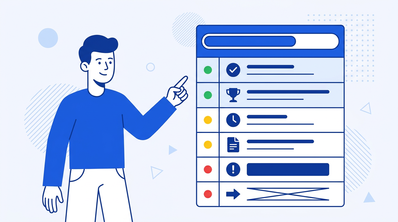
RAG Status with Conditional Formatting
RAG (Red, Amber, Green) status is the most useful signal in any project report. You can calculate it automatically based on due date and status:
Add a RAG column with this formula:
=IF(E2="Complete", "Green", IF(E2="Blocked", "Red", IF(D2<TODAY(), "Red", IF(D2<=TODAY()+7, "Amber", "Green"))))
Where E2 is Status and D2 is Due Date. Logic: Complete is always Green. Blocked is always Red. Overdue (past due date) is Red. Due within 7 days is Amber. Everything else is Green.
Now apply conditional formatting to color the RAG column: select it, go to Format, Conditional formatting, and add three rules — "Green" text gets green fill, "Amber" gets yellow, "Red" gets red.
Summary Section at the Top
Add a summary section above your task list (or on a separate summary tab) that gives the top-line view:
- Total tasks: =COUNTA(A5:A100)
- Complete: =COUNTIF(E5:E100, "Complete")
- In Progress: =COUNTIF(E5:E100, "In Progress")
- Blocked: =COUNTIF(E5:E100, "Blocked")
- Overdue: =COUNTIFS(E5:E100, "<>Complete", D5:D100, "<"&TODAY())
- % Complete: =COUNTIF(E5:E100, "Complete")/COUNTA(A5:A100)
Format the % Complete as a percentage. This summary gives stakeholders the full picture in six numbers.
Progress Bar
For a visual progress indicator, use a simple REPT formula:
=REPT("█", ROUND(B8*20, 0))&REPT("░", 20-ROUND(B8*20, 0))
Where B8 is your % Complete. This renders a text-based progress bar — crude but effective in a shared doc.
Filtering by Owner
Add a filter to your task list (Data, Create a filter) so each person can filter to just their tasks. Or create a named range and use FILTER to build a separate view per owner:
=FILTER(A5:F100, C5:C100=H1)
Where H1 is a cell containing the owner name. Change H1 to see any owner's tasks.
The Easy Way: Using SheetXAI in Google Sheets
Example 1: You have a task list already in the sheet.
"I have a task list on Sheet 1 with columns for task name, owner, start date, due date, and status. Build a project status report with RAG status, a summary section showing counts by status, and conditional formatting to highlight overdue and blocked tasks."
SheetXAI reads your data, adds the RAG formula, builds the summary section, and applies the conditional formatting.
Example 2: Your tasks live in a project management tool.
"Pull open tasks from our Asana project and build a status report showing tasks by owner and status, with RAG indicators and a summary of what's overdue or blocked."
SheetXAI connects to Asana, pulls the task data, and builds the full status report.
Try SheetXAI free and see what it builds for you.
Published May 2026. See also: How to Use Conditional Formatting in Google Sheets, How to Build a Budget vs. Actuals Report in Excel, and Google Sheets AI Guide.

